Introduction to the Monte Carlo technique
Monte Carlo simulations are in general a way to perform approximate solutions to complex problems by use of random sampling. The phrase "Monte Carlo" comes from the generous use of random numbers, which resembles the gambling of the famous Monaco casino, and the method was originally designed to facilitate calculations of neutron physics - more precisely for the Manhattan project. For the history of the Monte Carlo technique, we refer to an excellent essay by one of its inventors[1].
A simple example of Monte Carlo simulations
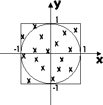
As an introduction, we consider a simple example. We intend to estimate the area of an object. For simplicity let us consider the unit circle, \(x^2 + y^2 \leq 1\), as shown in Figure xx--CrossReference--fig:MCcircle--xx. We now select \(N\) points randomly in the square of known area, \(A_{\rm s}=4\), that contains the circle fully. The area is defined by
\begin{equation}\label{dummy644155134} -1 \leq x \leq 1 \; \wedge \; -1 \leq y \leq 1 . \end{equation}
Each of the selected points inside this square are determined by retrieving independent, random values of \(x\) and \(y\) from a (pseudo-) random number generator. We will not here dwell on the issue of random number generation, which is described elsewhere[2], we only mention that such generators exist with specifications usefor for our purpose.
We now calculate the number of points, \(N_i\), that fall inside the unit circle. For large \(N\), the fraction of accepted points will according to the law of large numbers approach the ratio of the areas:
\begin{equation}\label{dummy702629630} \dfrac{N_i}{N} \rightarrow \dfrac{A_{\rm c}}{A_{\rm s}}. \end{equation}
Hence, this "numerical experiment" can be used to estimate the value of the circle area, \(A_{\rm c}\). Of course, the answer of this example is well known: The ratio is \(\pi/4\).
On Monte Carlo methods
Monte Carlo techniques can be used to solve problems much more complex than the example above. This may involve complex figures and/or a number of branches (choices between different possibilities). Here, analytical solutions are often impossible, making the Monte Carlo method show its full virtue.
In general, Monte Carlo techniques can be used for problems in different fields:
- In physics, the method can describe a number of many-body problems. E.g. in high-energy physics where a particle under consideration can be either absorbed, scattered, or converted into other particles.
- In mathematics, the method can be used to solve complex integrals in many dimensions with complex boundary conditions.
- In finance theory, the method is used to estimate the effect of uncertainties in market values.
- In computer science, the method has been used to optimize multi-variable functions.
Methods for variance reduction
As with all stochastical methods (including experiments), Monte Carlo methods are prone to statistical errors or variances. To reduce the statistical errors of simulations, a number of variance reduction methods have been designed. We here mention
- Stratified sampling. To ensure that the sampling is spread evenly, one would divide the parameter space up into mutually exclusive strata, and sample a given amount of each strata. In the circle example above, one could divide the area up into smaller quadrates and sample equally often from each.
- Importance sampling. When it can be shown that some places in parameter space is more crucial to the final result than others, one can chose to sample more often in the important regions. If the problem was e.g. to calculate the average height over sea level of a landscape, one would measure the mountain more careful than the lake, i.e. the Monte Carlo sampling would be denser at the mountain. In the stratified version of the circle example, one would sample more often in areas that contain a part of the circle rim, while completely filled or empty areas need little sampling.
Monte Carlo Ray-tracing
We will not explain the general Monte Carlo technique in further detail, but refer to a number of textbooks[3].
Rather, we specialize immediately to the method relevant for our purpose. This is known as Monte Carlo ray-tracing and can be performed to study objects which travel along a path (a ray), and can be (partially) absorbed or scattered into another direction, but not converted into other types of radiation. The most known example of this is light, and this type of ray-tracing is frequently used to generate realistic illumination in 3D computer graphics.
In a scientific environment, ray-tracing can be used to study non-interacting radiation, e.g. neutrons or X-rays. We will now dive into the explanation of ray-tracing simulations for this purpose.
- ↑ N. Metropolis. http://library.lanl.gov/la-pubs/00326866.pdf
- ↑ See the home page of the Mersenne Twister Algorithm http://www.math.sci.hiroshima-u.ac.jp/~m-mat/MT/emt.html
- ↑ D.P. Landau and K. Binder. A Guide to Monte Carlo Simulations in Statistical Physics. (Cambridge, 2005).
